Newton's Method for Constrained Optimization
We only consider convex optimization in this lecture.
Equality constraint
- Consider equality constrained optimization \begin{eqnarray*} &\text{minimize}& f(\mathbf{x}) \\ &\text{subject to}& \mathbf{A} \mathbf{x} = \mathbf{b}, \end{eqnarray*} where $f$ is convex.
KKT conditions
The Langrangian function is \begin{eqnarray*} L(\mathbf{x}, \nu) = f(\mathbf{x}) + \nu^T(\mathbf{A} \mathbf{x} - \mathbf{b}), \end{eqnarray*} where $\nu$ is the vector of Langrange multipliers.
Setting the gradient of Langrangian function to zero yields the optimality conditions: \begin{eqnarray*} \mathbf{A} \mathbf{x}^\star &=& \mathbf{b} \quad \quad (\text{primal feasibility condition}) \\ \nabla f(\mathbf{x}^\star) + \mathbf{A}^T \nu^\star &=& \mathbf{0} \quad \quad (\text{dual feasibility condition}) \end{eqnarray*}
Newton algorithm
Feasible start Newton
Let $\mathbf{x}$ be a feasible point, i.e., $\mathbf{A} \mathbf{x} = \mathbf{b}$. We determine the Newton direction $\Delta \mathbf{x}$ as follows.
By second order Taylor expansion \begin{eqnarray*} f(\mathbf{x} + \Delta \mathbf{x}) \approx f(\mathbf{x}) + \nabla f(\mathbf{x})^T \Delta \mathbf{x} + \frac 12 \Delta \mathbf{x}^T \nabla^2 f(\mathbf{x}) \Delta \mathbf{x}. \end{eqnarray*} To minimize the quadratic approximation subject to constraint $\mathbf{A}(\mathbf{x} + \Delta \mathbf{x}) = \mathbf{b}$, we solve the equality constrained QP: $$ \begin{array}{ll} \text{minimize} & f(\mathbf{x}) + \nabla f(\mathbf{x})^T \Delta \mathbf{x} + \frac 12 \Delta \mathbf{x}^T \nabla^2 f(\mathbf{x}) \Delta \mathbf{x}\\ \text{subject to} & \mathbf{A}\Delta \mathbf{x} = \mathbf{0} \end{array} $$ with variable $\Delta\mathbf{x}$. (Recall that $\mathbf{A}\mathbf{x} - \mathbf{b} = \mathbf{0}$. Without the equlity constraint, this is precisely what unconstrained Newton does.)
The KKT conditions for this QP are $$ \begin{split} \nabla^2 f(\mathbf{x})\Delta \mathbf{x} + \nabla f(\mathbf{x}) + \mathbf{A}^T\mathbf{w} &= 0 \\ \mathbf{A} \Delta \mathbf{x} &= \mathbf{0} \end{split} $$
In matrix form, $$ \begin{bmatrix} \nabla^2 f(\mathbf{x}) & \mathbf{A}^T \\ \mathbf{A} & \mathbf{0} \end{bmatrix} \begin{bmatrix} \Delta \mathbf{x} \\ \mathbf{w} \end{bmatrix} = \begin{bmatrix} -\nabla f(\mathbf{x}) \\ \mathbf{0} \end{bmatrix} $$ We solve this linear equation to find the Newton direction.
The matrix $$ \begin{bmatrix} \nabla^2 f(\mathbf{x}) & \mathbf{A}^T \\ \mathbf{A} & \mathbf{0} \end{bmatrix} $$ is called the KKT matrix.
When $\nabla^2 f(\mathbf{x})$ is pd and $\mathbf{A}$ has full row rank, the KKT matrix is nonsingular therefore the Newton direction is uniquely determined.
Line search is similar to the unconstrained case.
Infeasible start Newton
So far we have assumed that we start with a feasible point. How to derive Newton step from an infeasible point $\mathbf{x}$?
This only different from the feasible start method is that $\mathbf{A}\mathbf{x} - \mathbf{b} \neq \mathbf{0}$. Hence the KKT system is \begin{eqnarray*} \begin{bmatrix} \nabla^2 f(\mathbf{x}) & \mathbf{A}^T \\ \mathbf{A} & \mathbf{0} \end{bmatrix} \begin{bmatrix} \Delta \mathbf{x} \\ \mathbf{w} \end{bmatrix} = - \begin{bmatrix} \nabla f(\mathbf{x}) \\ \mathbf{A} \mathbf{x} - \mathbf{b} \end{bmatrix}. \end{eqnarray*} Writing the updated dual variable $\mathbf{w} = \nu + \Delta \nu$, we have the equivalent form in terms of primal update $\Delta \mathbf{x}$ and dual update $\Delta \nu$ \begin{eqnarray*} \begin{bmatrix} \nabla^2 f(\mathbf{x}) & \mathbf{A}^T \\ \mathbf{A} & \mathbf{0} \end{bmatrix} \begin{bmatrix} \Delta \mathbf{x} \\ \Delta \nu \end{bmatrix} = - \begin{bmatrix} \nabla f(\mathbf{x}) + \mathbf{A}^T \nu \\ \mathbf{A} \mathbf{x} - \mathbf{b} \end{bmatrix}. \end{eqnarray*} The righthand side is recognized as the primal and dual residuals (See the dual feasibility condition above). Therefore the infeasible Newton step is also interpreted as a primal-dual method, updating both the primal variable $\mathbf{x}$ and dual variable $\nu$ simultaneously.
It can be shown that the norm of the residuals decreases along the Newton direction. Therefore line search is based on the norm of residuals.
Inequality constraint - interior point method
Now consider the optimization problem with inequality constraints \begin{eqnarray*} &\text{minimize}& f_0(\mathbf{x}) \\ &\text{subject to}& f_i(\mathbf{x}) \le 0, \quad i = 1,\ldots,m \\ & & \mathbf{A} \mathbf{x} = \mathbf{b}, \end{eqnarray*} where $f_0, \ldots, f_m: \mathbb{R}^n \mapsto \mathbb{R}$ are convex and and twice continuously differentiable, and $\mathbf{A}$ has full row rank.
We assume the problem is solvable with optimal point $\mathbf{x}^\star$ and and optimal value $f_0(\mathbf{x}^\star) = p^\star$.
KKT conditions: \begin{eqnarray*} \mathbf{A} \mathbf{x}^\star = \mathbf{b}, f_i(\mathbf{x}^\star) &\le& 0, i = 1,\ldots,m \quad (\text{primal feasibility}) \\ \lambda^\star &\geq& \mathbf{0} \\ \nabla f_0(\mathbf{x}^\star) + \sum_{i=1}^m \lambda_i^\star \nabla f_i(\mathbf{x}^\star) + \mathbf{A}^T \nu^\star &=& \mathbf{0} \quad \quad \quad \quad \quad \quad (\text{dual feasibility}) \\ \lambda_i^\star f_i(\mathbf{x}^\star) &=& 0, \quad i = 1,\ldots,m. ~(\text{complementary slackness}) \end{eqnarray*}
Barrier method
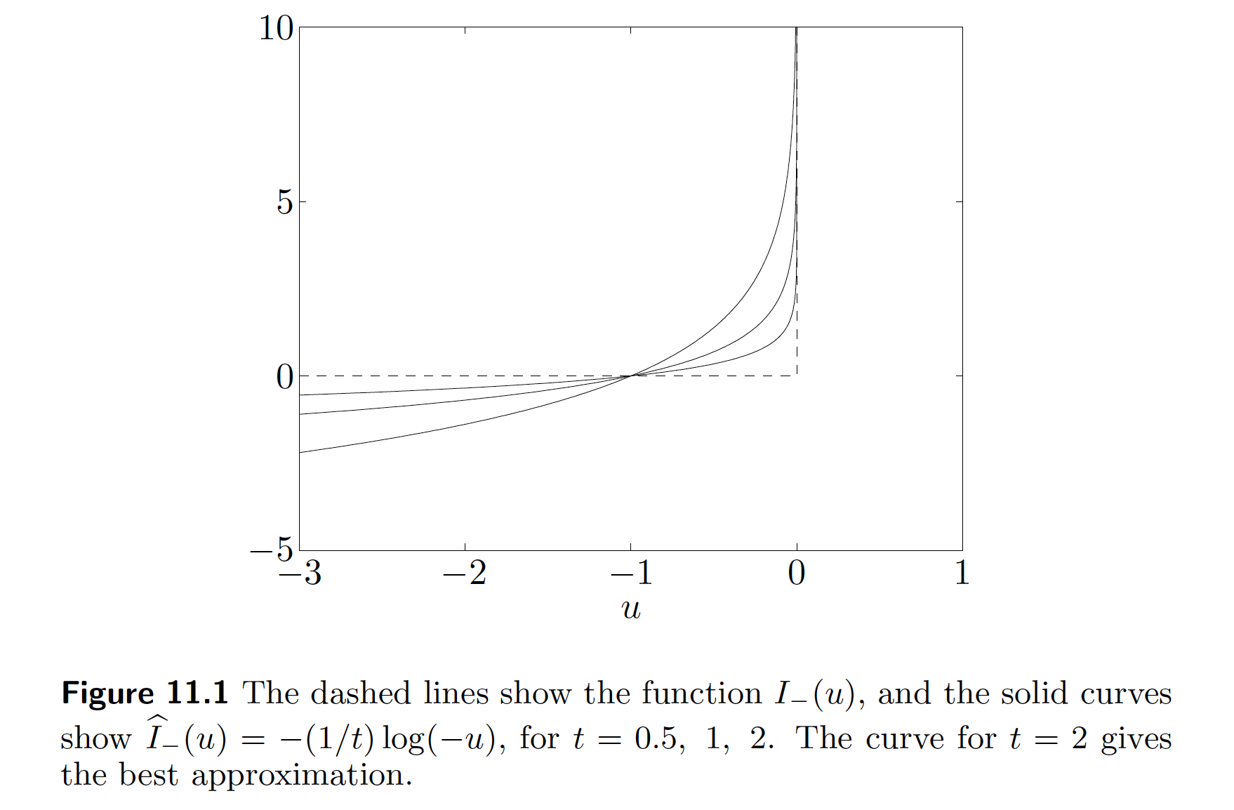
Alternative form makes inequality constraints implicit in the objective \begin{eqnarray*} &\text{minimize}& f_0(\mathbf{x}) + \sum_{i=1}^m \iota_-(f_i(\mathbf{x})) \\ &\text{subject to}& \mathbf{A} \mathbf{x} = \mathbf{b}, \end{eqnarray*} where \begin{eqnarray*} \iota_-(u) = \begin{cases} 0 & u \le 0 \\ \infty & u > 0 \end{cases} \end{eqnarray*} is the indicator function of the nonpositive half-line.
The idea of the barrier method is to approximate the nondifferentiable $\iota_-$ by a differentiable function \begin{eqnarray*} \hat\iota_-(u) = - (1/t) \log (-u), \quad u < 0, \end{eqnarray*} where $t>0$ is a parameter tuning the approximation accuracy. As $t$ increases, the approximation becomes more accurate.
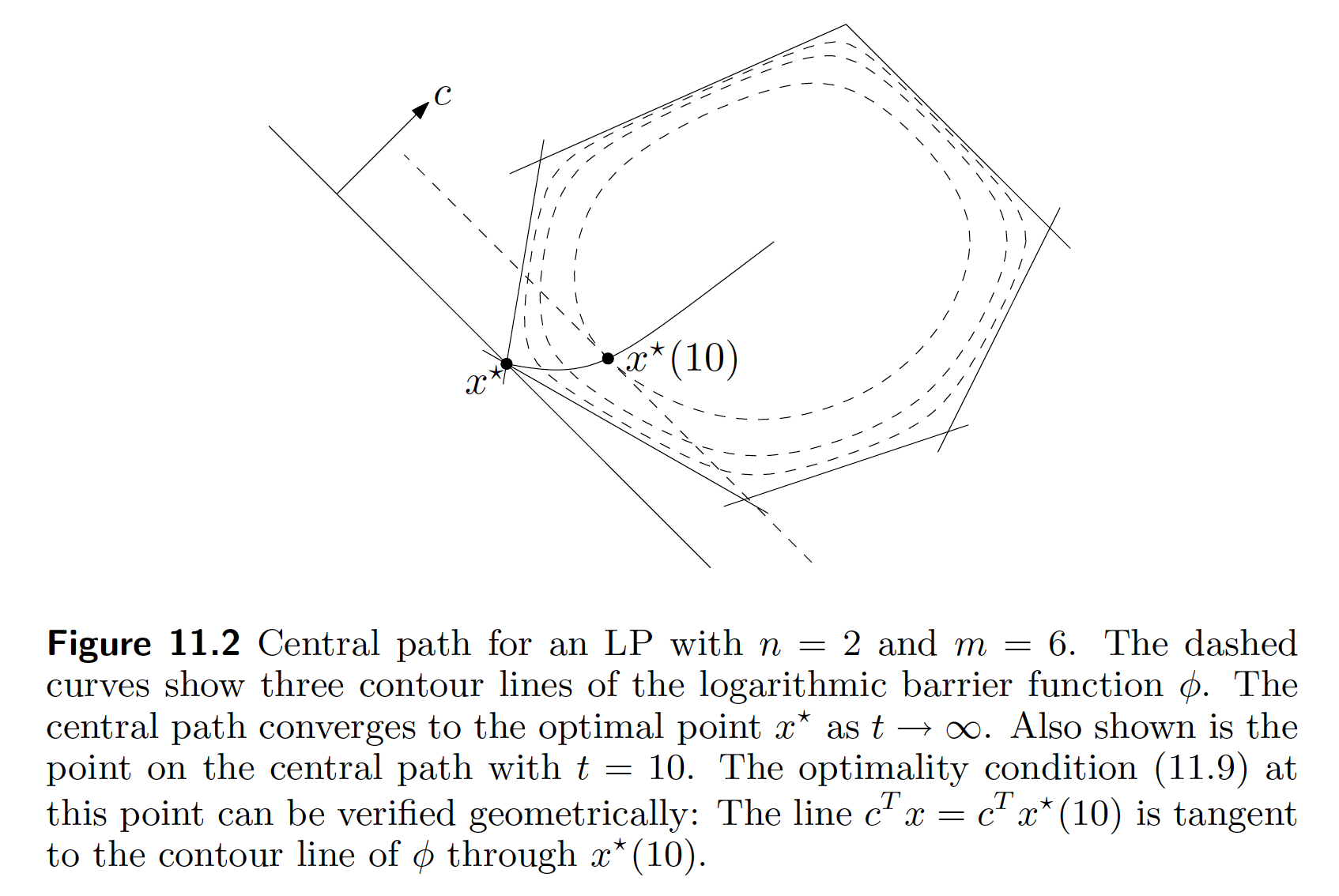
The barrier method solves a sequence of equality-constraint problems \begin{eqnarray*} &\text{minimize}& t f_0(\mathbf{x}) - \sum_{i=1}^m \log(-f_i(\mathbf{x})) \\ &\text{subject to}& \mathbf{A} \mathbf{x} = \mathbf{b}, \end{eqnarray*} for which we know how to solve from the above discussion, with the parameter $t$ increasing at each step and starting each equality-constrained Newton minimization at the solution for the previous value of $t$.
The function $\phi(\mathbf{x}) = - \sum_{i=1}^m \log (-f_i(\mathbf{x}))$ is called the logarithmic barrier or log barrier function.
Denote the solution at $t$ by $\mathbf{x}^\star(t)$. Using duality theory, it can be shown \begin{eqnarray*} f_0(\mathbf{x}^\star(t)) - p^\star \le m / t. \end{eqnarray*}
- Feasibility and phase I methods. Barrier method has to start from a strictly feasible point. We can find such a point by solving \begin{eqnarray*} &\text{minimize}& s \\ &\text{subject to}& f_i(\mathbf{x}) \le s, \quad i = 1,\ldots,m \\ & & \mathbf{A} \mathbf{x} = \mathbf{b} \end{eqnarray*} by the barrier method.
Primal-dual interior-point method
Difference from barrier method: no double loop (recall there is a inner mimnimization step).
In the barrier method, it can be shown that a point $\mathbf{x}$ is equal to $\mathbf{x}^\star(t)$ if and only if
$$ \begin{split} \nabla f_0(\mathbf{x}) + \sum_{i=1}^m \lambda_i \nabla f_i(\mathbf{x}) + \mathbf{A}^T \nu &= \mathbf{0} \\ -\lambda_i f_i(\mathbf{x}) &= 1/t, \quad i = 1,\ldots,m \\ \mathbf{A} \mathbf{x} &= \mathbf{b}. \end{split} $$
- We define the KKT residual
which we want to vanish, where
- Denote the current point and Newton step as
$$ \mathbf{y} = (\mathbf{x}, \lambda, \nu), \quad \Delta \mathbf{y} = (\Delta \mathbf{x}, \Delta \lambda, \Delta \nu). $$ In view of the linear equation $$ r_t(\mathbf{y} + \Delta \mathbf{y}) \approx r_t(\mathbf{y}) + Dr_t(\mathbf{y}) \Delta \mathbf{y} = \mathbf{0}, $$ we solve $\Delta \mathbf{y} = - D r_t(\mathbf{y})^{-1} r_t(\mathbf{y})$, i.e.,
for the primal-dual search direction.
References
- Boyd and Vandenberghe, 2004. Convex Optimization. Cambridge University Press (Chs. 10, 11).
Acknowledgment
Many parts of this lecture note is based on Dr. Hua Zhou's 2019 Spring Statistical Computing course notes available at http://hua-zhou.github.io/teaching/biostatm280-2019spring/index.html.