First-order Methods

Unconstrained optimization

• Problem $$ \min_{\mathbf{x}\in \mathbb{R}^d} f(\mathbf{x}) $$

• First-order optimality condition $$ \nabla f(\mathbf{x}^\star) = 0. $$

Gradient descent method

• Iteration:

$$ \boxed{ \mathbf{x}^{(t+1)} = \mathbf{x}^{(t)} - \gamma_t\nabla f(\mathbf{x}^{(t)}) } $$

for some step size $\gamma_t$. This is a special case of the Netwon-type algorithms with $\mathbf{H}_t = \mathbf{I}$ and $\Delta\mathbf{x} = \nabla f(\mathbf{x}^{(t)})$.

• Idea: iterative linear approximation (first-order Taylor series expansion).

$$ f(\mathbf{x}) \approx f(\mathbf{x}^{(t)}) + \nabla f(\mathbf{x}^{(t)})^T (\mathbf{x} - \mathbf{x}^{(t)}) $$

and then minimize the linear approximation within a compact set: let $\Delta\mathbf{x} = \mathbf{x}^{(t+1)}-\mathbf{x}^{(t)}$ to choose. Solve $$ \min_{\|\Delta\mathbf{x}\|_2 \le 1} \nabla f(\mathbf{x}^{(t)})^T\Delta\mathbf{x} $$ to obtain $\Delta\mathbf{x} = -\nabla f(\mathbf{x}^{(t)})/\|f(\mathbf{x}^{(t)})\|_2 \propto -\nabla f(\mathbf{x}^{(t)})$.

• Step sizes are chosen so that the descent property is maintained (e.g., line search).

  • Step size must be chosen at any time, since unlike Netwon's method, first-order approximation is always unbounded below.

• Pros

  • Each iteration is inexpensive.
  • No need to derive, compute, store and invert Hessians; attractive in large scale problems.

• Cons

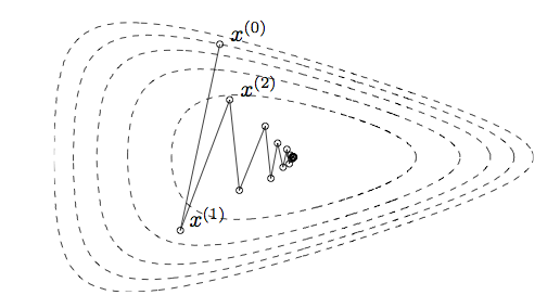
  • Slow convergence (zigzagging).

    

  • Do not work for non-smooth problems.

Convergence

• In general, the best we can obtain from gradient descent is linear convergence (cf. quadratic convergence of Newton).

• Example (Boyd & Vandenberghe Section 9.3.2) $$ f(\mathbf{x}) = \frac{1}{2}(x_1^2 + c x_2^2), \quad c > 1 $$ The optimal value is 0.

  It can be shown that if we start from $x^{(0)}=(c, 1)$, then $$ f(\mathbf{x}^{(t)}) = \left(\frac{c-1}{c+1}\right)^t f(\mathbf{x}^{(0)}) $$ and $$ \|\mathbf{x}^{(t)} - \mathbf{x}^{\star}\|_2 = \left(\frac{c-1}{c+1}\right)^t \|\mathbf{x}^{(0)} - \mathbf{x}^{\star}\|_2 $$

• More generally, if

  1. $f$ is convex and differentiable over $\mathbb{R}^d$;
  2. $f$ has $L$-Lipschitz gradients, i.e., $\|\nabla f(\mathbf{x}) - \nabla f(\mathbf{y})\|_2 \le L\|\mathbf{x} - \mathbf{y} \|_2$;

  3. $p^{\star} = \inf_{\mathbf{x}\in\mathbb{R}^d} f(x) > -\infty$ and attained at $\mathbf{x}^{\star}$,

     then $$ f(\mathbf{x}^{(t)}) - p^{\star} \le \frac{1}{2\gamma t}\|\mathbf{x}^{(0)} - \mathbf{x}^{\star}\|_2^2 = O(1/t). $$ for constant step size ($\gamma_t = \gamma \in (0, 1/L]$), a sublinear convergence. Similar upper bound with line search.

• If we further assume that $f$ is $\alpha$-strongly convex, i.e., $f(\mathbf{x}) - \frac{\alpha}{2}\|\mathbf{x}\|_2^2$ is convex for some $\alpha >0$, then $$ f(\mathbf{x}^{(t)}) - p^{\star} \le \frac{L}{2}\left(1 - \gamma\frac{2\alpha L}{\alpha + L}\right)^t \|\mathbf{x}^{(0)} - \mathbf{x}^{\star}\|_2^2 $$ and $$ \|\mathbf{x}^{(t)} - \mathbf{x}^{\star}\|_2^2 \le \left(1 - \gamma\frac{2\alpha L}{\alpha + L}\right)^t \|\mathbf{x}^{(0)} - \mathbf{x}^{\star}\|_2^2 $$ for constant step size $\gamma \in (0, 2/(\alpha + L) ]$.

Examples

• Least squares: $f(\mathbf{x}) = \frac{1}{2}\|\mathbf{A}\mathbf{x} - \mathbf{y}\|_2^2 = \frac{1}{2}\mathbf{x}^T\mathbf{A}^T\mathbf{A}\mathbf{x} - \mathbf{x}^T\mathbf{A}^T\mathbf{y} + \frac{1}{2}\mathbf{y}^T\mathbf{y}$

• Gradient $\nabla f(\mathbf{x}) = \mathbf{A}^T\mathbf{A}\mathbf{x} - \mathbf{A}^T\mathbf{y}$ is $\|\mathbf{A}^T\mathbf{A}\|_2$-Lipschitz. Hence $\gamma \in (0, 1/\sigma_{\max}(\mathbf{A})^2]$ guarantees descent property and convergence.

• If $\mathbf{A}$ is full column rank, then $f$ is also $\sigma_{\min}(\mathbf{A})^2$-strongly convex and the convergence is linear. Otherwise it is sublinear.

• Logistic regression: $f(\beta) = -\sum_{i=1}^n \left[ y_i \mathbf{x}_i^T \beta - \log (1 + e^{\mathbf{x}_i^T \beta}) \right]$

• Gradient $\nabla f(\beta) = - \mathbf{X}^T (\mathbf{y} - \mathbf{p})$ is $\frac{1}{4}\|\mathbf{X}^T\mathbf{X}\|_2$-Lipschitz.

• Even if $\mathbf{X}$ is full column rank, $f$ may not be strongly convex.

• Adding a ridge penalty $\frac{\rho}{2}\|\mathbf{x}\|_2^2$ makes the problems always strongly convex.

Accelerated gradient descent

First-order methods

• Iterative algorithm that generates sequence $\{\mathbf{x}^{(t)}\}$ such that $$ \mathbf{x}^{(t)} \in \mathbf{x}^{(0)} + \text{span}\{\nabla f(\mathbf{x}^{(0}), \dotsc, \nabla f(\mathbf{x}^{(t-1)})\}. $$

• Examples:

  • Gradient descent: $\mathbf{x}^{(t)} = \mathbf{x}^{(t-1)} - \gamma_t \nabla f(\mathbf{x}^{(t)})$.
  • Momentum method: $\mathbf{y}^{(t)} = \mathbf{x}^{(t-1)} - \gamma_t \nabla f(\mathbf{x}^{(t)})$, $\mathbf{x}^{(t)} = \mathbf{y}^{(t)} + \alpha_k (\mathbf{y}^{(t)} - \mathbf{y}^{(t-1)})$.

• In general, a first-order method generates
  $$ \mathbf{x}^{(t)} = \mathbf{x}^{(0)} - \sum_{k=1}^{t-1}\gamma_{t,k} \nabla f(\mathbf{x}^{(k)}) =: M_t(f,\mathbf{x}^{(0)}). $$

• Collection of all first-order method can be considered as the set of all $M_N$. Let's denote it by $\mathcal{M}_N$.

• Then we want to find a method $M_N\in\mathcal{M}_N$ that minimizes $$ \sup_{f\in\mathcal{F}} f(M_N(f,\mathbf{x}^{(0)})) - p^{\star}. $$ for a class of functions $\mathcal{F}$.

• Typically we choose the class of functions as $\mathcal{F}_L$, the set of functions satisfying the 3 assumptions used for convergence analysis of GD:

  1. $f$ is convex and differentiable over $\mathbb{R}^d$;
  2. $f$ has $L$-Lipschitz gradients, i.e., $\|\nabla f(\mathbf{x}) - \nabla f(\mathbf{y})\|_2 \le L\|\mathbf{x} - \mathbf{y} \|_2$;
  3. $p^{\star} = \inf_{\mathbf{x}\in\mathbb{R}^d} f(x) > -\infty$ and attained at $\mathbf{x}^{\star}$.

• We have seen that for gradient descent with a step size $1/L$, $$ \sup_{f\in\mathcal{F}_L} f(M_N(f,\mathbf{x}^{(0)})) - p^{\star} \le \frac{L}{2N}\|\mathbf{x}^{(0)} - \mathbf{x}^{\star}\|_2^2 = O(1/N). $$

• Nesterov (1983) showed that for $d \ge 2N + 1$ and every $\mathbf{x}^{(0)}$, there exists $f\in\mathcal{F}_L$ such that for any $M_N \in \mathcal{M}_N$, $$ f(\mathbf{x}^{(N)}) - p^{\star} \ge \frac{3L}{32(N+1)^2}\|\mathbf{x}^{(0)} - \mathbf{x}^{\star}\|_2^2. $$ suggesting that the minimax optimal rate of first order methods is at most $O(1/N^2)$.

• This also suggests that the $O(1/N)$ rate of GD can be improved.

• Nesterov's (1983) accelerated gradient method achieves the optimal rate: \begin{align*} \mathbf{y}^{(t+1)} &= \mathbf{x}^{(t)} - \frac{1}{L}\nabla f(\mathbf{x}^{(t)}) \\ \gamma_{t+1} &= \frac{1}{2}(1+\sqrt{1 + 4\gamma_t^2}) \\ \mathbf{x}^{(t+1)} &= \mathbf{y}^{(t+1)} + \frac{\gamma_t - 1}{\gamma_{t+1}}(\mathbf{y}^{(t+1)} - \mathbf{y}^{(t)}) \end{align*} with initializtion $\mathbf{y}^{(0)} = \mathbf{x}^{(0)}$ and $\gamma_0 = 1$.

• Theorem (Nesterov, 1983): Nesterov's accelerated gradient method algorithm satisfies $$ f(\mathbf{y}^{(t)}) - p^{\star} \le \frac{2L}{(t+1)^2}\|\mathbf{x}^{(0)} - \mathbf{x}^{\star}\|_2^2. $$ for $f\in\mathcal{F}_L$.

• Kim & Fessler's (2016) algorithm improved this rate by a factor of two: $$ f(\mathbf{x}^{(N)}) - p^{\star} \le \frac{L}{(N+1)^2} R^2 $$ for $f\in\mathcal{F}_L$ and $\|\mathbf{x}^{(0)} - \mathbf{x}^{\star}\|_2 \le R$.

Steepest descent method

• Recall the idea of GD: iterative linear approximation (first-order Taylor series expansion). $$ f(\mathbf{x}) \approx f(\mathbf{x}^{(t)}) + \nabla f(\mathbf{x}^{(t)})^T (\mathbf{x} - \mathbf{x}^{(t)}) $$ and then minimize the linear approximation within a compact set: $$ \min_{\|\Delta\mathbf{x}\|_2 \le 1} \nabla f(\mathbf{x}^{(t)})^T\Delta\mathbf{x}. $$

• The compact set need not be limitted to the $\ell_2$ norm ball in order to obtain a descent direction. For any unit norm ball, $$ \min_{\|\Delta\mathbf{x}\| \le 1} \nabla f(\mathbf{x}^{(t)})^T\Delta\mathbf{x} = - \|\nabla f(\mathbf{x}^{(t)})\|_{\ast} $$

• In particular, if $\ell_1$ norm ball is used, then $$ \min_{\|\Delta\mathbf{x}\|_1 \le 1} \nabla f(\mathbf{x}^{(t)})^T\Delta\mathbf{x} = - \|\nabla f(\mathbf{x}^{(t)})\|_{\infty} = - \max_{i=1,\dotsc, d} |[\nabla f(\mathbf{x}^{(t)})]_i| $$ and the descent direction is given by the convex hull of the elementary unit vectors corresponding to the coordinates of the maximum absolute derivatives. In other words, $$ \Delta\mathbf{x} = \sum_{i \in J} \alpha_i \text{sign}([\nabla f(\mathbf{x}^{(t)})]_i)\mathbf{e}_i, \quad \alpha_i \ge 0, ~ \sum_{i \in J} \alpha_i = 1, \quad J = \{j: |[\nabla f(\mathbf{x}^{(t)})]_j| = \|\nabla f(\mathbf{x}^{(t)})\|_{\infty} \}. $$

• Consider a linear regression setting. Assume each coordinate is standardized. If $\alpha_i = 1/|J|$ for $i \in J$, then the $\ell_1$-steepest descent update with a line search strategy of finding the maximal step size with which $J$ does not vary is the least angle regression (LAR). If only one coordinate is chosen and a very small step size $\epsilon$ is used, then this update is $\epsilon$-forward stagewise regression.

  

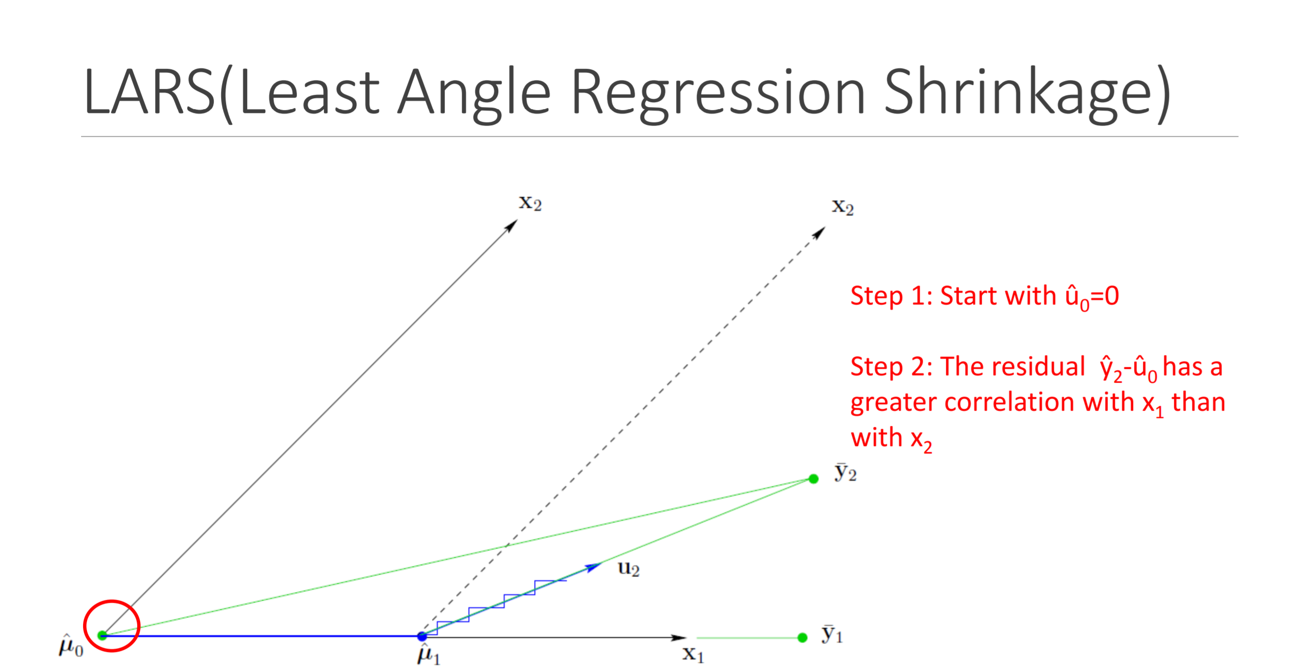
  Why these algorithms generate sparse solution paths should now be clear.

Proximal gradient methods

Constrained optimization

• Problem $$ \min_{\mathbf{x}\in C \subset \mathbb{R}^d} f(\mathbf{x}) = \min_{\mathbf{x}\in \mathbb{R}^d} f(\mathbf{x}) + \iota_C(\mathbf{x}) $$ where $\iota_C(\mathbf{x})$ is the indicator function of the constrained set $C$.

• Can be viewed as an unconstrained but nonsmooth problem.

• Recall that GD does not work for non-smooth problems. Need a new first-order method.

• Consider a genearalization $$ \min_{\mathbf{x}\in \mathbb{R}^d} f(\mathbf{x}) + g(\mathbf{x}) $$ where $f$ is smooth but $g$ is nonsmooth.

First-order optimality condition

• Assume convexity of $f$ and $g$. Then $\mathbf{x}^\star$ minimizes $f(\mathbf{x}) + g(\mathbf{x})$ if and only if $$ \nabla f(\mathbf{x}^\star) + \partial g(\mathbf{x}^\star) \ni 0, $$ where $\partial g(\mathbf{x})$ is the subdifferential of $g$ at $\mathbf{x}$: $$ \partial g(\mathbf{x}) = \{\mathbf{z}: g(\mathbf{y}) \ge g(\mathbf{x}) + \langle \mathbf{z}, \mathbf{y} - \mathbf{x} \rangle, ~ \forall \mathbf{y} \in \mathbb{R}^d \}. $$ Vector $\mathbf{z} \in \partial g(\mathbf{x})$ is called a subgradient of $g$ at $\mathbf{x}$. (Example: $g(x)=|x|$. $\partial g(0) = [-1, 1]$.)

Proximal gradient

• Proximal gradient solves the nonsmooth first-order opitimality condition in the same spirit as GD.

• Motivation: alternative view of GD $$ \mathbf{x}^{(t+1)} = \mathbf{x}^{(t)} - \gamma_t\nabla f(\mathbf{x}^{(t)}) = \arg\min_{\mathbf{x}\in\mathbb{R}^d} \left\{ f(\mathbf{x}^{(t)}) + \langle \nabla f(\mathbf{x}^{(t)}), \mathbf{x} - \mathbf{x}^{(t)} \rangle + \frac{1}{2\gamma_t}\|\mathbf{x} - \mathbf{x}^{(t)}\|_2^2 \right\} $$ Thus consider \begin{align*} \mathbf{x}^{(t+1)} &= \arg\min_{\mathbf{x}\in\mathbb{R}^d} \left\{ f(\mathbf{x}^{(t)}) + \langle \nabla f(\mathbf{x}^{(t)}), \mathbf{x} - \mathbf{x}^{(t)} \rangle + \frac{1}{2\gamma_t}\|\mathbf{x} - \mathbf{x}^{(t)}\|_2^2 + g(\mathbf{x}) \right\} \\ &= \arg\min_{\mathbf{x}\in\mathbb{R}^d} \left\{ \gamma_t g(\mathbf{x}) + \frac{1}{2}\|\mathbf{x} - [\mathbf{x}^{(t)} - \gamma_t\nabla f(\mathbf{x}^{(t)}) ]\|_2^2 \right\}. \end{align*}

• The map $$ \mathbf{x} \mapsto \arg\min_{\mathbf{y}\in\mathbb{R}^d} \left\{ \phi(\mathbf{y}) + \frac{1}{2}\|\mathbf{y} - \mathbf{x} \|_2^2 \right\} $$ is called the proximal map, proximal operator, or proximity operator of $\phi$, denoted by $$ \mathbf{prox}_{\phi}(\mathbf{x}). $$

• Thus the new update rule is $$ \boxed{\mathbf{x}^{(t+1)} = \mathbf{prox}_{\gamma_t g}\left(\mathbf{x}^{(t)} - \gamma_t\nabla f(\mathbf{x}^{(t)})\right)} $$ and called the proximal gradient method.

Proximal maps

• A key to success of the proximal gradient method is the ease of evaluation of the proximal map $\mathbf{prox}_{\gamma g}(\cdot)$. Often proximal maps have closed-form solutions.

• Examples

  1. If $g(\mathbf{x}) \equiv 0$, then $\mathbf{prox}_{\gamma g}(\mathbf{x}) = \mathbf{x}$. PG reduces to GD.
  2. If $g(\mathbf{x}) = \iota_C(\mathbf{x})$ for a closed convex set $C$, then $\mathbf{prox}_{\gamma g}(\mathbf{x}) = P_C(\mathbf{x})$, or the orthogonal projection of $\mathbf{x}$ to set $C$. Proximal gradient reduces to projected gradient.
  3. If $g(\mathbf{x}) = \lambda\|\mathbf{x}\|_1$, then $\mathbf{prox}_{\gamma g}(\mathbf{x}) = S_{\lambda\gamma}(\mathbf{x}) = (\text{sign}(x_i)(|x_i| - \lambda\gamma))_{i=1}^d$, the soft-thresholding operator.
  4. If $g(\mathbf{x}) = \lambda\|\mathbf{x}\|_2$, then $$ \mathbf{prox}_{\gamma g}(\mathbf{x}) = \begin{cases} (1 - \lambda\gamma/\|\mathbf{x}\|_2)\mathbf{x}, & \|\mathbf{x}\|_2 \ge \lambda\gamma \\ \mathbf{0}, & \text{otherwise} \end{cases} $$
  5. If $g(\mathbf{X}) = \lambda\|\mathbf{X}\|_*$ (nuclear norm), then $\mathbf{prox}_{\gamma g}(\mathbf{X}) = \mathbf{U}\text{diag}((\sigma_1 - \lambda\gamma)_+, \dotsc, (\sigma_r - \lambda\gamma)_+)\mathbf{V}^T$, when the SVD of $\mathbf{X}$ is $\mathbf{X} = \mathbf{U}\text{diag}(\sigma_1, \dotsc, \sigma_r)\mathbf{V}^T$.

• Lasso $$ \min_{\beta} \frac{1}{2}\|\mathbf{y} - \mathbf{X}\beta\|_2^2 + \lambda\|\beta\|_1 $$

  • $f(\beta) = \frac{1}{2}\|\mathbf{y} - \mathbf{X}\beta\|_2^2$, $\nabla f(\beta) = \mathbf{X}^T(\mathbf{X}\beta - \mathbf{y})$
  • $g(\beta) = \lambda\|\beta\|_1$.
  • Update rule: $\beta^{(t+1)} = S_{\lambda\gamma_t}\left(\beta^{(t)} - \gamma_t \mathbf{X}^T(\mathbf{X}\beta^{(t)} - \mathbf{y})\right)$. Can be computed in parallel (including matrix-vector multiplications).

Convergence

• It can be shown that if

  1. $f$ is convex and differentiable over $\mathbb{R}^d$;
  2. $f$ has $L$-Lipschitz gradients, i.e., $\|\nabla f(\mathbf{x}) - \nabla f(\mathbf{y})\|_2 \le L\|\mathbf{x} - \mathbf{y} \|_2$;
  3. $g$ is a closed convex function (i.e., $\mathbf{epi} f$ is closed);
  4. $p^{\star} = \inf_{\mathbf{x}\in\mathbb{R}^d} f(x) + g(x) > -\infty$ and attained at $\mathbf{x}^{\star}$.

  then proximal gradient method converges to an optimal solution, at the same rate (in terms of objective values) as GD. For example, with a constant step size $\gamma_t = \gamma =1/L$, $$ f(\mathbf{x}^{(t)}) + g(\mathbf{x}^{(t)}) - p^{\star} \le \frac{L}{2t}\|\mathbf{x}^{(0)} - \mathbf{x}^{\star}\|_2^2. $$ A similar rate holds with backtracking.

• If $f$ or $g$ is strongly convex, linear convergence.

FISTA: accelerated proximal gradient

• Fast Iterative Shrinkage-Thresholding Algorithm (Beck & Tebolle, 2009)

\begin{align*} \mathbf{y} &= \mathbf{x}^{(t)} + \frac{t-1}{t+2}(\mathbf{x}^{(t)} − \mathbf{x}^{(t−1)}) \\ \mathbf{x}^{(t+1)} &= \mathbf{prox}_{\gamma_t g}(\mathbf{y} - \gamma_t \nabla g(\mathbf{y}) ) \end{align*}

with initialization $\mathbf{x}^{(-1)} = \mathbf{x}^{(0)}$.

• Proximal gradient version of Nesterov's (1983) accelerated gradient algorithm.

• Under the above assumptions and with a constant step size $\gamma_t = \gamma =1/L$, $$ f(\mathbf{x}^{(N)}) + g(\mathbf{x}^{(N)}) - p^{\star} \le \frac{L}{2(N+1)^2}\|\mathbf{x}^{(0)} - \mathbf{x}^{\star}\|_2^2. $$

Mirror descent method

• Again, constrained optimization problem $$ \min_{\mathbf{x}\in C \subset \mathbb{R}^d} f(\mathbf{x}). $$

• Second alternative view of GD \begin{align*} \mathbf{x}^{(t+1)} = \mathbf{x}^{(t)} - \gamma_t\nabla f(\mathbf{x}^{(t)}) &= \arg\min_{\mathbf{x}\in\mathbb{R}^d} \left\{ f(\mathbf{x}^{(t)}) + \langle \nabla f(\mathbf{x}^{(t)}), \mathbf{x} - \mathbf{x}^{(t)} \rangle + \frac{1}{2\gamma_t}\|\mathbf{x} - \mathbf{x}^{(t)}\|_2^2 \right\} \\ &= \arg\min_{\mathbf{x}\in\mathbb{R}^d} \left\{ \langle \nabla f(\mathbf{x}^{(t)}), \mathbf{x}\rangle + \frac{1}{2\gamma_t}\|\mathbf{x} - \mathbf{x}^{(t)}\|_2^2 \right\} \end{align*}

• or projected (proximal) gradient \begin{align*} \mathbf{x}^{(t+1)} = P_C\left( \mathbf{x}^{(t)} - \gamma_t\nabla f(\mathbf{x}^{(t)}) \right) &= P_C\left( \arg\min_{\mathbf{x}\in\mathbb{R}^d} \left\{ \langle \nabla f(\mathbf{x}^{(t)}), \mathbf{x}\rangle + \frac{1}{2\gamma_t}\|\mathbf{x} - \mathbf{x}^{(t)}\|_2^2 \right\} \right) \end{align*}

• This relies too much on the (Euclidean) geometry of $\mathbb{R}^d$: $\|\cdot\|_2 = \langle \cdot, \cdot \rangle$.

• If the distance measure $\frac{1}{2}\|\mathbf{x} - \mathbf{y}\|_2^2$ is replaced by something else (say $d(\mathbf{x}, \mathbf{y})$) that better reflects the geometry of $C$, then update such as $$ \mathbf{x}^{(t+1)} = P_C^{d}\left( \arg\min_{\mathbf{x}\in \mathbb{R}^d} \left\{ \langle \nabla f(\mathbf{x}^{(t)}), \mathbf{x}\rangle + \frac{1}{\gamma_t}d(\mathbf{x}, \mathbf{x}^{(t)}) \right\} \right) $$ may converge faster. Here, $$ P_C^d(\mathbf{y}) = \arg\min_{\mathbf{x}\in C} d(\mathbf{x}, \mathbf{y}) $$ to reflect the geometry.

Bregman divergence

• Let $\phi: \mathcal{X} \to \mathbb{R}$ be a continuously differentiable, strictly convex function defined on a vector space $\mathcal{X} \subset \mathbb{R}^d$. The Bregman divergence with respect to $\phi$ is defined by $$ B_{\phi}(\mathbf{x}\Vert \mathbf{y}) = \phi(\mathbf{x}) - \phi(\mathbf{y}) - \langle \nabla\phi(\mathbf{y}), \mathbf{x} - \mathbf{y} \rangle $$

• It can be shown that $B_{\phi}(\mathbf{x}\Vert \mathbf{y}) \ge 0$ and $B_{\phi}(\mathbf{x}\Vert \mathbf{y}) = 0 \iff \mathbf{x}=\mathbf{y}$. But $B_{\phi}(\mathbf{x}\Vert \mathbf{y}) \neq B_{\phi}(\mathbf{y}\Vert \mathbf{x})$ in general.

• Examples

  • $\phi(\mathbf{x}) = \frac{1}{2}\|\mathbf{x}\|_2^2$, $\mathcal{X}=\mathbb{R}^d$: $B_{\phi}(\mathbf{x}\Vert\mathbf{y}) = \frac{1}{2}\|\mathbf{x} - \mathbf{y}\|_2^2$.
  • $\phi(\mathbf{x}) = \sum_{i=1}^d x_i\log x_i - \sum_{i=1}^d x_i$, $\mathcal{X}=\mathbb{R}_{++}^d$ (generalized negative entropy): $B_{\phi}(\mathbf{x}\Vert\mathbf{y}) = \sum_{i=1}^d x_i\log\frac{x_i}{y_i} - \sum_{i=1}^d x_i - \sum_{i=1}^d y_i$ (generalized Kullback-Leibler divergence).
  • $\phi(\mathbf{X}) = -\log\det\mathbf{X}$, $\mathcal{X} = \mathbb{S}_{++}^d$: $B_{\phi}(\mathbf{X}, \mathbf{Y}) = \mathbf{tr}(\mathbf{X}\mathbf{Y}^{-1}) - d - \log\det(\mathbf{X}\mathbf{Y}^{-1})$ (log-det divergence).

• If $\phi$ is $\alpha$-strongly convex with respect to norm $\|\cdot\|$, i.e., $$ \phi(\mathbf{y}) \ge \phi(\mathbf{x}) + \langle \nabla\phi(\mathbf{y}, \mathbf{y} - \mathbf{x} \rangle + \frac{\alpha}{2}\|\mathbf{y} - \mathbf{x}\|^2, $$ then $$ B_{\phi}(\mathbf{x}\Vert\mathbf{y}) \ge \frac{\alpha}{2}\|\mathbf{x} - \mathbf{y}\|^2. $$

  • Negative entropy is 1-strongly convex with respect to $\|\cdot\|_1$.

• Projection onto $C\subset \mathcal{X}$ under the Bregman divergence $$ P_C^{\phi}(\mathbf{y}) = \arg\min_{\mathbf{x}\in C} B_{\phi}(\mathbf{x}\Vert\mathbf{y}) = \arg\min_{\mathbf{x}\in C} \left\{ \phi(\mathbf{x}) - \phi(\mathbf{y}) - \langle \nabla\phi(\mathbf{y}), \mathbf{x} - \mathbf{y} \rangle \right\} = \arg\min_{\mathbf{x}\in C} \left\{ \phi(\mathbf{x}) - \langle \nabla\phi(\mathbf{y}), \mathbf{x} \rangle \right\} $$

Mirror descent

• Minimization over a closed convex set $C \subset \mathcal{X}$ by: \begin{align*} \mathbf{x}^{(t+1)} &= P_C^{\phi}\left( \arg\min_{\mathbf{x}\in\mathbb{R}^d} \left\{ \langle \nabla f(\mathbf{x}^{(t)}), \mathbf{x}\rangle + \frac{1}{2\gamma_t}B_{\phi}(\mathbf{x}\Vert\mathbf{x}^{(t)}) \right\} \right) \\ &= P_C^{\phi}\left( \arg\min_{\mathbf{x}\in\mathbb{R}^d} \left\{ \gamma_t\langle \nabla f(\mathbf{x}^{(t)}), \mathbf{x}\rangle + \phi(\mathbf{x}) - \phi(\mathbf{x}^{(t)}) - \langle \nabla\phi(\mathbf{x}^{(t)}), \mathbf{x} - \mathbf{x}^{(t)} \rangle \right\} \right)\\ &= P_C^{\phi}\left( \arg\min_{\mathbf{x}\in\mathbb{R}^d} \left\{\phi(\mathbf{x}) - \langle \nabla\phi(\mathbf{x}^{(t)}) - \gamma_t \nabla f(\mathbf{x}^{(t)}), \mathbf{x} \rangle \right\} \right). \end{align*}

• In the inner (unconstrained) minimization step, the optimiality condition is $$ \nabla \phi(\mathbf{x}) = \nabla\phi(\mathbf{x}^{(t)}) - \gamma_t \nabla f(\mathbf{x}^{(t)}) $$ If $\phi$ is strongly convex, then this is equivalent to $$ \mathbf{x} = \nabla \phi^*\left(\nabla\phi(\mathbf{x}^{(t)}) - \gamma_t \nabla f(\mathbf{x}^{(t)}) \right), $$ where $\phi^*(\cdot)$ is the Fenchel conjugate function of $\phi$: $$ \phi^*(\mathbf{y}) = \sup_{\mathbf{x}\in\mathbb{R}^d} \langle \mathbf{x}, \mathbf{y} \rangle - \phi(\mathbf{x}) $$ (assuming $\phi(\mathbf{x}) = \infty$ if $\mathbf{x} \notin \mathcal{X}$).

  • If $\phi(\cdot)$ is strongly convex, $\phi^*(\cdot)$ is differentiable. Hence $\nabla\phi^*(\cdot)$ is well-defined. Furthermore, $\nabla\phi^*(\nabla\phi(\mathbf{x}))=\mathbf{x})$.

• Hence a mirror descent iteration consists of: \begin{align*} \mathbf{y}^{(t+1)} &= \nabla\phi(\mathbf{x}^{(t)}) - \gamma_t \nabla f(\mathbf{x}^{(t)}) \quad \text{(gradient step)} \\ \tilde{\mathbf{x}}^{(t+1)} &= \nabla \phi^*(\mathbf{y}^{(t+1)}) \quad \text{(mirroring step)} \\ \mathbf{x}^{(t+1)} &= P_C^{\phi}(\tilde{\mathbf{x}}^{(t+1)}) \quad \text{(projection step)} \end{align*}

• Technically speaking, gradients $\nabla\phi(\mathbf{x})$, $\nabla f(\mathbf{x})$ lie in the dual vector space $\mathcal{X}^*$ of $\mathcal{X}$. Therefore a gradient step should be taken in the dual space. (If $\mathcal{X}=\mathbb{R}^d$, then $\mathcal{X}^*=\mathcal{X}$. That's why $\mathbf{x}^{(t+1)} = \mathbf{x}^{(t)} - \gamma_t\nabla f(\mathbf{x}^{(t)})$ is valid in GD.) So mirror descent first maps a primal point $\mathbf{x}$ to its dual point $\phi(\mathbf{x})$, takes a gradient step, and maps it back to the primal space by inverse mapping $\nabla\phi^*(\mathbf{y}) = (\nabla\phi)^{-1}(\mathbf{y})$.

• Actual computation can be simplified, since \begin{align*} \mathbf{x}^{(t+1)} &= P_C^{\phi}\left( \arg\min_{\mathbf{x}\in\mathbb{R}^d} \left\{\phi(\mathbf{x}) - \langle \nabla\phi(\mathbf{x}^{(t)}) - \gamma_t \nabla f(\mathbf{x}^{(t)}), \mathbf{x} \rangle \right\} \right) \\ &= P_C^{\phi}(\tilde{\mathbf{x}}^{(t+1)}) \\ &= \arg\min_{\mathbf{x}\in C} \left\{ \phi(\mathbf{x}) - \langle \nabla\phi(\tilde{\mathbf{x}}^{(t+1)}), \mathbf{x} \rangle \right\} \\ &= \arg\min_{\mathbf{x}\in C} \left\{ \phi(\mathbf{x}) - \langle \mathbf{y}^{(t+1)}, \mathbf{x} \rangle \right\} \\ &= \arg\min_{\mathbf{x}\in C} \left\{ \phi(\mathbf{x}) - \langle \nabla\phi(\mathbf{x}^{(t)}) - \gamma_t \nabla f(\mathbf{x}^{(t)}), \mathbf{x} \rangle \right\}. \end{align*} Compare the first and the last lines.

• Convergence rates are similar to GD, with smaller constants.

Mirror descent example

• Optimization over probability simplex $\Delta^{d-1} = \{\mathbf{x}\in\mathcal{X}=\mathbb{R}_{++}^d: \sum_{i=1}^d x_i = 1\}$.

• Appropriate Bregman divergence: Kullback-Leibler. $\phi(\mathbf{x}) = \sum_{i=1}^d x_i\log x_i - \sum_{i=1}^d x_i$.

  • Fact: $\phi(\cdot)$ is 1-strongly convex with respect to $\|\cdot\|_1$. (Pinsker's inequality)
  • $\nabla\phi(\mathbf{x}) = (\log x_1, \dotsc, \log x_d)^T = \log\mathbf{x}$.
  • $\nabla\phi^*(\mathbf{y}) = (\nabla\phi)^{-1}(\mathbf{y}) = (e^{y_1}, \dotsc, e^{y_d})^T = \exp(\mathbf{y})$.
  • Update: \begin{align*} \mathbf{y}^{(t+1)} &= \log\mathbf{x}^{(t)} - \gamma_t\nabla f(\mathbf{x}^{(t)}) \\ \tilde{\mathbf{x}}^{(t+1)} &= \exp\left(\log\mathbf{x}^{(t)} - \gamma_t\nabla f(\mathbf{x}^{(t)}) \right) \\ \mathbf{x}^{(t+1)} &= \exp\left(\log\mathbf{x}^{(t)} - \gamma_t\nabla f(\mathbf{x}^{(t)}) \right)/Z_t \\ &= \mathbf{x}^{(t)}\exp\left(- \gamma_t\nabla f(\mathbf{x}^{(t)}) \right)/Z_t, \quad Z_t = \sum_{i=1}^d {x}_i^{(t)}\exp\left(- \gamma_t\nabla f(\mathbf{x}^{(t)})_i \right) = \mathbf{1}^T\exp\left(\log\mathbf{x}^{(t)} - \gamma_t\nabla f(\mathbf{x}^{(t)}) \right), \end{align*}
  • The last step is because $$ P_{\Delta^{d-1}}^{\phi}(\mathbf{y}) = \arg\min_{\mathbf{x}\in\Delta^{d-1}} KL(\mathbf{x}\Vert\mathbf{y}) = \arg\min_{x_i \ge 0, \sum_{i=1}^d x_i=1} \sum_{i=1}^d\left(x_i\log\frac{x_i}{y_i} - x_i + y_i\right) = \arg\min_{x_i \ge 0, \sum_{i=1}^d x_i=1} \sum_{i=1}^d\left(x_i\log\frac{x_i}{y_i}\right). $$ Lagrangian $$ \mathcal{L}(\mathbf{x}, \mu) = \sum_{i=1}^d \left(x_i\log\frac{x_i}{y_i}\right) + \mu\left(\sum_{i=1}^d x_i - 1\right) $$ yields $$ \log\frac{x_i}{y_i} + 1 + \mu = 0 \quad \iff \quad x_i = y_i\exp(-\mu-1) = c y_i, ~ c > 0, \quad i=1, \dotsc, d. $$ Summing up yields $c = 1/(\sum_{i=1}^d y_i)$ to have $$ x_i = \frac{y_i}{\sum_{j=1}^d y_j}, \quad i=1,\dotsc, d. $$
  • This special case is called the exponentiated gradient method.

References

• Boyd and Vandenberghe, 2004. Convex Optimization. Cambridge University Press. (Ch. 9)

• Nesterov, Y. (1983). A method of solving a convex programming problem with convergence rate O(1/k2). Soviet Mathematics Doklady, 27(2):372–376.

• Efron, B., Hastie, T., Johnstone, I., & Tibshirani, R. (2004). Least angle regression. The Annals of statistics, 32(2), 407-499.

• Beck, A. and Teboulle, M. (2009). A fast iterative shrinkage-thresholding algorithm for linear inverse problems. SIAM J. Imaging Sci., 2(1):183–202.

• Kim, D., & Fessler, J. A. (2016). Optimized first-order methods for smooth convex minimization. Mathematical programming, 159(1-2), 81-107.

• Juditsky, A., & Nemirovski, A. (2011). First order methods for nonsmooth convex large-scale optimization, I: general purpose methods. Optimization for Machine Learning, 121-148.