MM Algorithms
Lange, Kenneth, David R. Hunter, and Ilsoon Yang. "Optimization transfer using surrogate objective functions" (with discussion). Journal of Computational and Graphical Statistics 9, no. 1 (2000): 1-20.
![]()
"MM" stands for either majorization-minimization or minorization-maximization. For the origination, see the discussion by Xiaoli Meng and rejoinder by Lange and Hunter in the Lange, Hunter, & Yang (2000) paper.
For minimization of $f(\mathbf{x})$ - majorization-minimization.
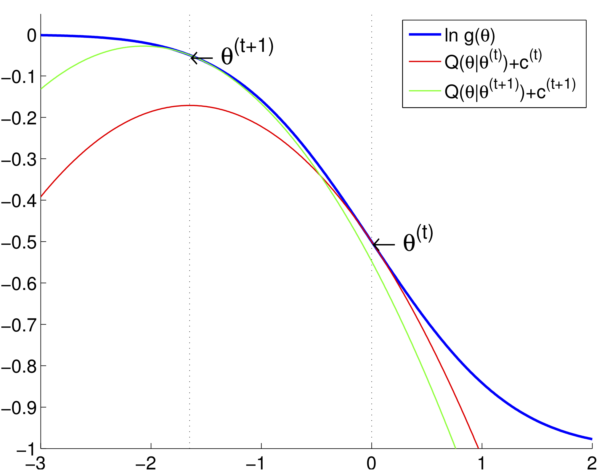
- Majorization step: Construct a surrogate function $g(\mathbf{x}|\mathbf{x}^{(t)})$ that satisfies $$ \begin{eqnarray*} f(\mathbf{x}) &\le& g(\mathbf{x}|\mathbf{x}^{(t)}) \quad \text{(dominance condition)} \\ f(\mathbf{x}^{(t)}) &=& g(\mathbf{x}^{(t)}|\mathbf{x}^{(t)}) \quad \text{(tangent condition)}. \end{eqnarray*} $$
- Minimization step: $$ \mathbf{x}^{(t+1)} = \text{argmin}_{\mathbf{x}} \, g(\mathbf{x}|\mathbf{x}^{(t)}). $$
For maximization of $f(\mathbf{x})$ - minorization-maximization.
- Minorization step: Construct a surrogate function $g(\mathbf{x}|\mathbf{x}^{(t)})$ that satisfies $$ \begin{eqnarray*} f(\mathbf{x}) &\ge& g(\mathbf{x}|\mathbf{x}^{(t)}) \quad \text{(dominance condition)} \\ f(\mathbf{x}^{(t)}) &=& g(\mathbf{x}^{(t)}|\mathbf{x}^{(t)}) \quad \text{(tangent condition)}. \end{eqnarray*} $$
- Maximization step: $$ \mathbf{x}^{(t+1)} = \text{argmax}_{\mathbf{x}} \, g(\mathbf{x}|\mathbf{x}^{(t)}). $$

- Descent property (for minorization-maximization) is guaranteed:
$$
f(\mathbf{x}^{(t)}) = g(\mathbf{x}^{(t)}|\mathbf{x}^{(t)}) \ge g(\mathbf{x}^{(t+1)}|\mathbf{x}^{(t)}) \ge f(\mathbf{x}^{(t+1)}).
$$
- The first inequality is because $\mathbf{x}^{(t+1)}$ minimizes $g(\mathbf{x}|\mathbf{x}^{(t)})$.
- Full minimization of $g(\mathbf{x}|\mathbf{x}^{(t)})$ is not essential.
MM examples
Coordinate descent
- Idea: coordinate-wise minimization is often easier than the full-dimensional minimization $$ x_j^{(t+1)} = \arg\min_{x_j} f(x_1^{(t+1)}, \dotsc, x_{j-1}^{(t+1)}, x_j, x_{j+1}^{(t)}, \dotsc, x_d^{(t)}) $$

Similar to the Gauss-Seidel method for solving linear equations.
Block descent: a vector version of coordinate descent $$ \mathbf{x}_j^{(t+1)} = \arg\min_{\mathbf{x}_j} f(\mathbf{x}_1^{(t+1)}, \dotsc, \mathbf{x}_{j-1}^{(t+1)}, \mathbf{x}_j, \mathbf{x}_{j+1}^{(t)}, \dotsc, \mathbf{x}_d^{(t)}) $$
MM interpretation: consider simplest two-block case: $$ \min_{(\mathbf{x}, \mathbf{y})} g(\mathbf{x}, \mathbf{y}) = \min_{\mathbf{x}}\min_{\mathbf{y}} g(\mathbf{x}, \mathbf{y}). $$
- Set $f(\mathbf{x}) = \min_{\mathbf{y}} g(\mathbf{x}, \mathbf{y})$
- Let $\mathbf{y}^{(t)} = \arg\min_{\mathbf{y}} g(\mathbf{x}^{(t)}, \mathbf{y})$
- Then $$ f(\mathbf{x}) = \min_{\mathbf{y}} g(\mathbf{x}, \mathbf{y}) \le g(\mathbf{x}, \mathbf{y}^{(t)}) = g(\mathbf{x}, \arg\min_{\mathbf{y}} g(\mathbf{x}^{(t)}, \mathbf{y}) ) =: h(\mathbf{x}|\mathbf{x}^{(t)}) $$ and $$ f(\mathbf{x}^{(t)}) = \min_{\mathbf{y}} g(\mathbf{x}^{(t)}, \mathbf{y}) = g(\mathbf{x}, \mathbf{y}^{(t)}) = g(\mathbf{x}^{(t)}, \arg\min_{\mathbf{y}} g(\mathbf{x}^{(t)}, \mathbf{y}) ) = h(\mathbf{x}^{(t)}|\mathbf{x}^{(t)}) $$
- Thus $h(\mathbf{x}|\mathbf{x}^{(t)})$ is a majorizing function.
Q: why objective value converges?
- A: descent property
Caution: even if the objective function is convex, coordinate descent may not converge to the global minimum and converge to a suboptimal point.

Fortunately, if the objective function is convex and differentible, or a sum of differentible convex function and seperable nonsmooth convex function, i.e., $$ h(\mathbf{x}) = f(\mathbf{x}) + \sum_{i=1}^d g_i(x_i), $$ where $f$ is convex and differentiable and $g_i$ are convex but not necessarily differentiable, then CD converges to the global minimum.
See
Tseng, Paul. "Convergence of a block coordinate descent method for nondifferentiable minimization." Journal of optimization theory and applications 109, no. 3 (2001): 475-494. https://doi.org/10.1023/A:1017501703105
for more details.
- GLMNET uses CD to solve lasso-related optimization problems.
EM algorithm
Dempster, Arthur P., Nan M. Laird, and Donald B. Rubin. "Maximum likelihood from incomplete data via the EM algorithm." Journal of the Royal Statistical Society: Series B (Methodological) 39, no. 1 (1977): 1-22.
Baum, Leonard E., Ted Petrie, George Soules, and Norman Weiss. "A maximization technique occurring in the statistical analysis of probabilistic functions of Markov chains." Annals of Mathematical Statistics 41, no. 1 (1970): 164-171.
EM is a special case of the MM algorithm.
Goal: to maximize the log-likelihood of the observed data $\mathbf{o}$ (usual MLE)
Difficulty: log-likelihood is not obvious to how increase (e.g., presence of missing data)
Idea: choose missing data $\mathbf{Z}$ such that MLE for the complete data is easy.
Let $p_{\theta}(\mathbf{o},\mathbf{z})$ be the density of the complete data. The the marginal loglikelihood to be maximized with respect to parameter $\theta$ is $$ \ell(\theta) = \log \int p_\theta(\mathbf{o}, \mathbf{z}) d\mathbf{z}. $$
Then, \begin{align*} \ell(\theta) &= \log \int p_\theta (\mathbf{o}, \mathbf{z}) d\mathbf{z} = \log \int \frac{p_\theta (\mathbf{o}) p_\theta (\mathbf{z}|\mathbf{o})}{p_{\theta^{(t)}}(\mathbf{z}|\mathbf{o})} p_{\theta^{(t)}} (\mathbf{z}|\mathbf{o}) d\mathbf{z} \\ & \ge \int \log \left[\frac{p_\theta(\mathbf{o}) p_\theta (\mathbf{z}|\mathbf{o})}{p_{\theta^{(t)}} (\mathbf{z}| \mathbf{o})}\right] p_{\theta^{(t)}}(\mathbf{z}|\mathbf{o}) d\mathbf{z} \\ &= \int \log \left[p_\theta (\mathbf{o},\mathbf{z})\right]p_{\theta^{(t)}} (\mathbf{z}|\mathbf{o}) d\mathbf{z} - \int \log \left[p_{\theta^{(t)}} (\mathbf{z}|\mathbf{o})\right] p_{\theta^{(t)}} (\mathbf{z} |\mathbf{o}) d\mathbf{z} \\ &= Q(\theta | \theta^{(t)}) - \int \log \left[p_{\theta^{(t)}} (\mathbf{z}|\mathbf{o})\right] p_{\theta^{(t)}} (\mathbf{z}|\mathbf{o}) d\mathbf{z} \end{align*} where $p_{\theta} (\mathbf{z} | \mathbf{o})$ is the conditional density of $\mathbf{Z}$ given (observed) data $\mathbf{o}$, and $$ Q(\theta | \theta^{(t)}) = \int \log \left[p_\theta (\mathbf{o}, \mathbf{z})\right] p_{\theta^{(t)}} (\mathbf{z} | \mathbf{o}) d\mathbf{z} =: \mathbb{E}_{\mathbf{Z}|\mathbf{X}}^{(t)} \left[\log p_\theta(\mathbf{o}, \mathbf{z})\right] $$ is the conditional expecation of the complete likelihood with respect to the current conditional density $p_{\theta^{(t)}} (\mathbf{z} | \mathbf{o})$.
The key inequality in the above derivation is Jensen's inequality: equality holds if and only if $p_{\theta} (\mathbf{z} | \mathbf{o})=p_{\theta^{(t)}} (\mathbf{z} | \mathbf{o})$, i.e., $\theta=\theta^{(t)}$.
Thus $Q(\theta | \theta^{(t)}) - \int \log \left[p_{\theta^{(t)}} (\mathbf{z}|\mathbf{o})\right] p_{\theta^{(t)}} (\mathbf{z}|\mathbf{o}) d\mathbf{z}$ satisfies both the dominance and tangent conditions, and is a legitimate surrogate function for minorization-maximization of $\ell(\theta)$.
However, since the second term is irrelavent to $\theta$, we can use the first part only: $Q(\theta | \theta^{(t)})$.
Now we have a compact two-step iterative procedure:
- E step: calculate the conditional expectation $$ Q(\theta | \theta^{(t)}) = \mathbb{E}_{\mathbf{Z}|\mathbf{X}}^{(t)} \left[\log p_\theta(\mathbf{o}, \mathbf{z})\right] $$
- M step: maximize $Q(\theta|\theta^{(t)})$ to generate the next iterate $$ \theta^{(t+1)} = \text{argmax}_{\theta} \, Q(\theta|\theta^{(t)}) $$
Again, full maximization is not necessary (generalized EM).
Example: MLE of multivariate $t$ distribution parameters
$\mathbf{W} \in \mathbb{R}^{p}$ has a multivariate $t$-distribution $t_p(\mu,\Sigma,\nu)$ with mean $\mu$, covariance $\Sigma$, and degrees of freedom $\nu$ if $\mathbf{W}|\{U=u\} \sim \mathcal{N}(\mu, u^{-1}\Sigma)$ and $U \sim \text{Gamma}\left(\frac{\nu}{2}, \frac{\nu}{2}\right)$.
Widely used for robust modeling (heavier tail than normal).
Recall Gamma($\alpha,\beta$) has density \begin{eqnarray*} f(u \mid \alpha,\beta) = \frac{\beta^{\alpha} u^{\alpha-1}}{\Gamma(\alpha)} e^{-\beta u}, \quad u \ge 0, \end{eqnarray*} with mean $\mathbf{E}(U)=\alpha/\beta$, and $\mathbf{E}(\log U) = \psi(\alpha) - \log \beta$, where $\psi(x)=\Gamma'(x)/\Gamma(x)$ is the digamma function.
Density of $\mathbf{W}$ is \begin{eqnarray*} f_p(\mathbf{w} \mid \mu, \Sigma, \nu) = \frac{\Gamma \left(\frac{\nu+p}{2}\right) \text{det}(\Sigma)^{-1/2}}{(\pi \nu)^{p/2} \Gamma(\nu/2) [1 + \delta (\mathbf{w},\mu;\Sigma)/\nu]^{(\nu+p)/2}}, \end{eqnarray*} where \begin{eqnarray*} \delta (\mathbf{w},\mu;\Sigma) = (\mathbf{w} - \mu)^T \Sigma^{-1} (\mathbf{w} - \mu) \end{eqnarray*} is the squared Mahalanobis distance between $\mathbf{w}$ and $\mu$.
Given i.i.d. data $\mathbf{w}_1, \ldots, \mathbf{w}_n$, the log-likelihood is \begin{eqnarray*} \ell(\mu, \Sigma, \nu) &=& - \frac{np}{2} \log (\pi \nu) + n \left[ \log \Gamma \left(\frac{\nu+p}{2}\right) - \log \Gamma \left(\frac{\nu}{2}\right) \right] \\ && - \frac n2 \log \det \Sigma + \frac n2 (\nu + p) \log \nu \\ && - \frac{\nu + p}{2} \sum_{j=1}^n \log [\nu + \delta (\mathbf{w}_j,\mu;\Sigma) ] \end{eqnarray*} How to compute the MLE $(\hat \mu, \hat \Sigma, \hat \nu)$?
$\mathbf{W}_j | \{U_j=u_j\}$ are independently $\mathcal{N}(\mu,\Sigma/u_j)$, and $U_j$ are i.i.d. $\text{Gamma}\left(\frac{\nu}{2},\frac{\nu}{2}\right)$.
Observed data $\mathbf{o}=(\mathbf{w}_1,\dotsc,\mathbf{w}_n)$. Missing data: $\mathbf{z}=(u_1,\ldots,u_n)^T$.
Log-likelihood of the complete data is \begin{eqnarray*} L_c (\mu, \Sigma, \nu) &=& - \frac{np}{2} \ln (2\pi) - \frac{n}{2} \log \det \Sigma \\ & & - \frac 12 \sum_{j=1}^n u_j (\mathbf{w}_j - \mu)^T \Sigma^{-1} (\mathbf{w}_j - \mu) \\ & & - n \log \Gamma \left(\frac{\nu}{2}\right) + \frac{n \nu}{2} \log \left(\frac{\nu}{2}\right) \\ & & + \frac{\nu}{2} \sum_{j=1}^n (\log u_j - u_j) - \sum_{j=1}^n \log u_j. \end{eqnarray*}
Since $\text{Gamma}(\alpha,\beta)$ is the conjugate prior for the normal-gamma model, the conditional distribution of $U$ given $\mathbf{W} = \mathbf{w}$ is $\text{Gamma}((\nu+p)/2, (\nu + \delta(\mathbf{w},\mu; \Sigma))/2)$. Thus \begin{eqnarray*} \mathbf{E} (U_j \mid \mathbf{w}_j, \mu^{(t)},\Sigma^{(t)},\nu^{(t)}) &=& \frac{\nu^{(t)} + p}{\nu^{(t)} + \delta(\mathbf{w}_j,\mu^{(t)};\Sigma^{(t)})} =: u_j^{(t)} \\ \mathbf{E} (\log U_j \mid \mathbf{w}_j, \mu^{(t)},\Sigma^{(t)},\nu^{(t)}) &=& \log u_j^{(t)} + \left[ \psi \left(\frac{\nu^{(t)}+p}{2}\right) - \log \left(\frac{\nu^{(t)}+p}{2}\right) \right]. \end{eqnarray*}
The surrogate $Q$ function takes the form (up to an additive constant)
Maximization over $(\mu, \Sigma)$ is simply a weighted multivariate normal problem \begin{eqnarray*} \mu^{(t+1)} &=& \frac{\sum_{j=1}^n u_j^{(t)} \mathbf{w}_j}{\sum_{j=1}^n u_j^{(t)}}, \quad \left( u_j^{(t)} = \frac{\nu^{(t)} + p}{\nu^{(t)} + \delta(\mathbf{w}_j,\mu^{(t)};\Sigma^{(t)})}\right) \\ \Sigma^{(t+1)} &=& \frac 1n \sum_{j=1}^n u_j^{(t)} (\mathbf{w}_j - \mu^{(t+1)}) (\mathbf{w}_j - \mu^{(t+1)})^T. \end{eqnarray*} Notice down-weighting of outliers is obvious in the update.
Maximization over $\nu$ is a univariate problem - can be done with golden section or bisection.
From EM to MM
- Recall our picture for understanding the ascent property of EM
- Questions:
- Is EM principle only limited to maximizing likelihood model?
- Can we flip the picture and apply same principle to minimization problem?
- Is there any other way to produce such surrogate function?
Example: t-distribution revisited
Recall that given i.i.d. data $\mathbf{w}_1, \ldots, \mathbf{w}_n$ from $p$-variate $t$-distribution $t_p(\mu,\Sigma,\nu)$, the log-likelihood is \begin{eqnarray*} \ell(\mu, \Sigma, \nu) &=& - \frac{np}{2} \log (\pi \nu) + n \left[ \log \Gamma \left(\frac{\nu+p}{2}\right) - \log \Gamma \left(\frac{\nu}{2}\right) \right] + \frac n2 (\nu + p) \log \nu \\ && - \frac n2 \log \det \Sigma - \frac{\nu + p}{2} \sum_{j=1}^n \log [\nu + \delta (\mathbf{w}_j,\mu;\Sigma) ]. \end{eqnarray*}
Early on we discussed EM algorithm for maximizing the log-likelihood.
To derive an alternative MM algorithm, note that \begin{align*} & - \frac n2 \log \det \Sigma - \frac{\nu + p}{2} \sum_{j=1}^n \log [\nu + \delta (\mathbf{w}_j,\mu;\Sigma) ] \\ &= \sum_{j=1}^n \left( -\frac{1}{2} \log \det \Sigma - \frac{\nu + p}{2} \log [\nu + \delta (\mathbf{w}_j,\mu;\Sigma) ] \right) \end{align*}
We minorize each summand: \begin{align*} & -\frac{1}{2} \log \det \Sigma - \frac{\nu + p}{2} \log [\nu + \delta (\mathbf{w}_j,\mu;\Sigma) ] \\ &= - \frac{\nu + p}{2} \log\left((\det\Sigma)^{1/(\nu + p)}[\nu + \delta (\mathbf{w}_j,\mu;\Sigma) ] \right) \\ &\ge -\frac{u_j^{(t)}}{2(\det\Sigma^{(t)})^{1/(\nu + p)}}\left((\det\Sigma)^{1/(\nu + p)}[\nu + \delta (\mathbf{w}_j,\mu;\Sigma) ] \right) + c_j^{(t)} \end{align*} using the convexity of $-\log: -\log u \ge -\log v - (u - v)/v$. Set $v=(\det\Sigma^{(t)})^{1/(\nu^{(t)} + p)}[\nu^{(t)} + \delta (\mathbf{w}_j,\mu^{(t)};\Sigma^{(t)})]$. The $c_j^{(t)}$ is the term irrelevant to optimization.
- This yields a new surrogate function (different from the $Q$ function above)
Now we can deploy the block ascent strategy.
Fixing $\nu$, it can be shown that update of $\mu$ and $\Sigma$ are given by \begin{eqnarray*} \mu^{(t+1)} &=& \frac{\sum_{j=1}^n u_j^{(t)} \mathbf{w}_j}{\sum_{j=1}^n u_j^{(t)}}, \quad \left( u_j^{(t)} = \frac{\nu^{(t)} + p}{\nu^{(t)} + \delta(\mathbf{w}_j,\mu^{(t)};\Sigma^{(t)})}\right) \\ \Sigma^{(t+1)} &=& \frac{1}{\sum_{i=1}^n u_i^{(t)}} \sum_{j=1}^n u_j^{(t)} (\mathbf{w}_j - \mu^{(t+1)}) (\mathbf{w}_j - \mu^{(t+1)})^T. \end{eqnarray*}
Fixing $\mu$ and $\Sigma$, we can update $\nu$ by univariate maximization of $g(\mu^{(t+1)}, \Sigma^{(t+1)}, \nu)$.
- For more details, see
Wu, Tong Tong, and Kenneth Lange. "The MM alternative to EM." Statistical Science 25, no. 4 (2010): 492-505. https://doi.org/10.1214/08-STS264
MM example: nonnegative matrix factorization (NMF)
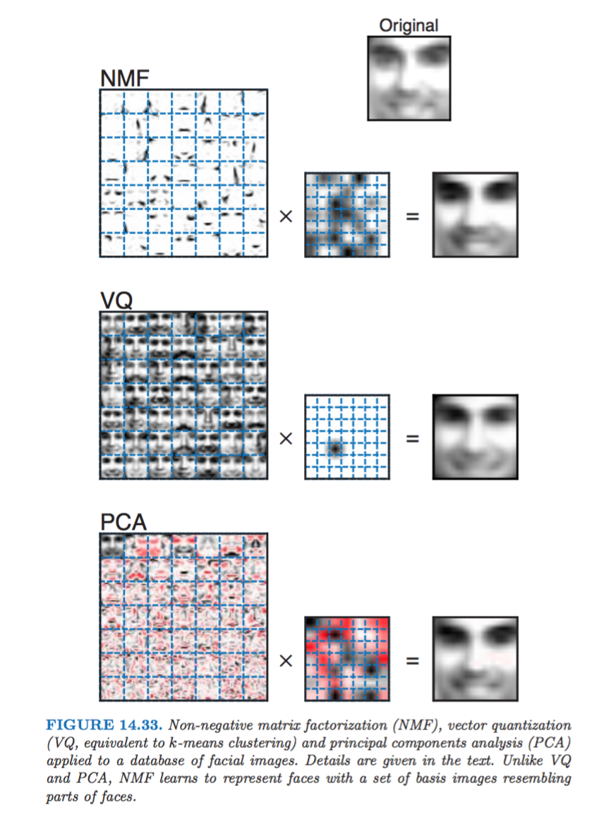
NMF was introduced by Lee and Seung (1999, 2001) as an analog of principal components and vector quantization with applications in data compression and clustering.
In mathematical terms, one approximates a data matrix $\mathbf{X} \in \mathbb{R}^{m \times n}$ with nonnegative entries $x_{ij}$ by a product of two low-rank matrices $\mathbf{V} \in \mathbb{R}^{m \times r}$ and $\mathbf{W} \in \mathbb{R}^{r \times n}$ with nonnegative entries $v_{ik}$ and $w_{kj}$.
Consider minimization of the squared Frobenius norm $$ L(\mathbf{V}, \mathbf{W}) = \|\mathbf{X} - \mathbf{V} \mathbf{W}\|_{\text{F}}^2 = \sum_i \sum_j \left( x_{ij} - \sum_k v_{ik} w_{kj} \right)^2, \quad v_{ik} \ge 0, w_{kj} \ge 0, $$ which should lead to a good factorization.
$L(\mathbf{V}, \mathbf{W})$ is not convex, but bi-convex. The strategy is to alternately update $\mathbf{V}$ and $\mathbf{W}$.
The key is the majorization, via convexity of the function $(x_{ij} - x)^2$, $$ \left( x_{ij} - \sum_k v_{ik} w_{kj} \right)^2 \le \sum_k \frac{a_{ikj}^{(t)}}{b_{ij}^{(t)}} \left( x_{ij} - \frac{b_{ij}^{(t)}}{a_{ikj}^{(t)}} v_{ik} w_{kj} \right)^2, $$ where $$ a_{ikj}^{(t)} = v_{ik}^{(t)} w_{kj}^{(t)}, \quad b_{ij}^{(t)} = \sum_k v_{ik}^{(t)} w_{kj}^{(t)}. $$
This suggests the alternating multiplicative updates $$ \begin{eqnarray*} v_{ik}^{(t+1)} &=& v_{ik}^{(t)} \frac{\sum_j x_{ij} w_{kj}^{(t)}}{\sum_j b_{ij}^{(t)} w_{kj}^{(t)}} \\ b_{ij}^{(t+1/2)} &=& \sum_k v_{ik}^{(t+1)} w_{kj}^{(t)} \\ w_{kj}^{(t+1)} &=& w_{kj}^{(t)} \frac{\sum_i x_{ij} v_{ik}^{(t+1)}}{\sum_i b_{ij}^{(t+1/2)} v_{ik}^{(t+1)}}. \end{eqnarray*} $$ (Homework).
The update in matrix notation is extremely simple $$ \begin{eqnarray*} \mathbf{B}^{(t)} &=& \mathbf{V}^{(t)} \mathbf{W}^{(t)} \\ \mathbf{V}^{(t+1)} &=& \mathbf{V}^{(t)} \odot (\mathbf{X} \mathbf{W}^{(t)T}) \oslash (\mathbf{B}^{(t)} \mathbf{W}^{(t)T}) \\ \mathbf{B}^{(t+1/2)} &=& \mathbf{V}^{(t+1)} \mathbf{W}^{(t)} \\ \mathbf{W}^{(t+1)} &=& \mathbf{W}^{(t)} \odot (\mathbf{X}^T \mathbf{V}^{(t+1)}) \oslash (\mathbf{B}^{(t+1/2)T} \mathbf{V}^{(t)}), \end{eqnarray*} $$ where $\odot$ denotes elementwise multiplication and $\oslash$ denotes elementwise division. If we start with $v_{ik}, w_{kj} > 0$, parameter iterates stay positive.
Monotoniciy of the algorithm is free (from MM principle).
Summary
Rationale of the MM principle for developing optimization algorithms
- Free the derivation from missing data structure.
- Avoid matrix inversion.
- Linearize an optimization problem.
- Deal gracefully with certain equality and inequality constraints.
- Turn a non-differentiable problem into a smooth problem.
- Separate the parameters of a problem (perfect for massive, fine-scale parallelization).
Generic methods for majorization and minorization - inequalities
- Jensen's (information) inequality - EM algorithms
- Supporting hyperplane property of a convex function
- The Cauchy-Schwartz inequality - multidimensional scaling
- Arithmetic-geometric mean inequality
- Quadratic upper bound principle - Bohning and Lindsay
- ...
A comprehensive reference for MM algorithms is
Lange, Kenneth. MM optimization algorithms. Vol. 147. SIAM, 2016.

Acknowledgment
Many parts of this lecture note is based on Dr. Hua Zhou's 2019 Spring Statistical Computing course notes available at http://hua-zhou.github.io/teaching/biostatm280-2019spring/index.html.